On the interpretation and presentation of
“chained (2007) dollars”
2018-08-14
Introduction
The concept of “chained (2007) dollars”, as used for example in Statistics Canada Table 36-10-0104-01, can be difficult to understand and is sometimes misinterpreted. This short note explains the history behind the way this concept has been used by Statistics Canada and provides guidance on how the published “chained (2007) dollars” time series should be perceived, reported and charted.
Post-war history: Fixed-weighted volume and price indexes
Statistics Canada began releasing estimates of gross national product (GNP) in the late 1940s. In those days the central concept in the national accounts was GNP, rather than gross domestic product (GDP) as today. GNP measures the income/output of Canadian-owned factors of production, no matter the country in which the production occurs, while GDP measures the income/output of factors of production that are resident in Canada, no matter the country of residence of their owners. The main points discussed in this note have nothing to do with whether the central aggregate is GNP or GDP.
Initially the estimates were made available only in current prices. Then in the early 1950s the agency began releasing the estimates with a breakdown in terms of ‘value’, ‘volume’ and ‘price’. This breakdown was such that the relative change in GNP at current prices was equal to the relative change in a GNP volume index times the relative change in a GNP price index:
(1) GNP(t)/GNP(s)=K(t)/K(s)*P(t)/P(s)
where t and s indicate time periods (months, quarters or years).
In this decomposition K and P are both indexes and their scale (level) is arbitrary. GNP is, of course, measured in dollars but K and P both have no unique units of measure. Only the relative changes in K and P have meaning. This makes sense when one thinks about it because the individual transactions making up GNP are extremely heterogeneous, consisting of billions of different goods and services. What common unit of measure could possibly be conceived for purposes of aggregating the levels of all these products in physical/volume terms or in terms of prices?
Users of the accounts found and still find this decomposition of GNP relative changes into volume and price components very useful because it shows how changes in the magnitude of GNP can be interpreted as the net result of ‘real growth’ and ‘inflation’. For example, if GNP grew by 3 per cent, the indexes might decompose this growth into 1.6 per cent real growth and 1.4 per cent inflation as follows:
(2) 1.03000=1.01600*1.01378
From the beginning, the Laspeyres index number formula – a base-weighted formula – was used to calculate the volume index and the Paasche formula – a current-weighted formula – to calculate the price index. Since the two indexes were chained only infrequently – every ten years or so initially – the Laspeyres volume measure had the convenient property that if it was scaled to be the same as nominal GNP in the base year (the year in which the index weights were chosen), then the volume estimates could be interpreted as “GNP measured in the constant prices of the base year”. Thus, the volume index estimates came to be known as “GNP at constant prices of the base year” or “real GNP measured in base year prices”.
The level of this index had an intuitive meaning only because (1) the index number formula was the one proposed by Laspeyres, (2) the arbitrary scale factor was nominal GNP in the base year and (3) the index weights were updated and linked infrequently. One could interpret real GNP in some year t as being the sum of the values of all transactions during year t, measured not in the prices of year t, but rather in the “fixed” prices of the index base year. In other words, the volume index numbers for the different components of GNP – household consumption expenditure, government expenditure and so on – were additive to total GNP. This additivity was a very convenient property.
This can be seen with some Laspeyres arithmetic. The Laspeyres volume index formula is:
(3) K(t)=∑k(t)*p(b)/∑k(b)*p(b)
where k(t) and p(t) are the quantity and price for transactions in item i in period t and the summations are over all items i. (The i subscripts are omitted for simplicity of presentation.) The denominator is the value of all transactions in the base period b, valued in the prices of period b, and the numerator is the value of all transactions in period t, valued in the prices of period b. As written here, the volume index K(t) is scaled to equal 1 in the base period b, that is K(b) = 1. If the index is rescaled by multiplying by the value of GNP in the base period the scale factor is, in effect, the same as the denominator. Accordingly the rescaled volume index can then be interpreted as the quantities purchased in period t valued at the prices of period b, or in other words GNP at the constant prices of period b. The volume indexes for the components of real GNP are therefore additive.
The point here is that because of rather particular circumstances, the volume index level actually has a meaningful interpretation. In almost any other circumstances the volume level would have no easy interpretation. The use of another index number formula, such as those proposed by Fisher or Tornqvist, or a more frequent updating and chaining of the index weights, such as annually or quarterly, or a different index number scaling factor in the base year, such as 100, would invalidate this interpretation and the indexes would no longer be additive.
One of the particular circumstances just mentioned is the requirement that the weights and the associated base year be held constant for a significant period of time. This period was chosen to be “about ten years” initially. The “constant prices of the base year” interpretation and the associated additivity property only held true in the time interval after the base year. When a rebasing was done, updating the base year and the associated weights to a more recent year, the new GNP volume series was linked (chained) to the old one to provide a continuous time series. Each component of GNP, and each sub-component of each component, had to be linked separately. This meant that real GNP was not additive - and the “constant prices of the base year” interpretation was invalid - for all years prior to the base year. Users of the statistics were gratified that the more recent real GNP numbers were additive, but they were often perplexed that the numbers for years prior to the base year were not. Since the national accounts are “accounts”, people thought they should always “add up properly”. To alleviate these concerns, the practice was adopted, from early on, that “adjusting entry” time series were introduced into the GNP tables. They were calculated as the arithmetic differences between each aggregate and its corresponding linked components. There were hundreds of these – essentially meaningless – adjusting entries in the national accounts database. When they were included as components of GNP, the accounts then “added up properly”.
The 1980s and 1990s: Cautious steps
In 1986 Statistics Canada adopted GDP as its main aggregate, instead of GNP. This change had no impact on the volume-price decomposition per se. The existing practice that was being used to calculate real growth and inflation during the GNP era was simply continued for GDP.
However, a more relevant (from the perspective of this note) change during the 1980s is that the rebasing period was changed from “about ten years” to “about five years”. This change was necessitated by increasingly large and frequent fluctuations in relative prices – such as the relative prices for energy, high-tech and agricultural products – which meant the base year’s price configuration became less and less relevant, more and more quickly. This illustrates the dilemma that came with the post-war fixed-weights deflation approach. Everyone liked the additivity feature, but no one liked the fact that the base year was becoming more quickly irrelevant to more current circumstances. Why, for example, would users of the national accounts in 1987 be interested to see GDP restated in the prices of the mid-1970s when those prices were so different? More frequent rebasing meant more relevant deflation, but it also meant a much shorter period within which the volume accounts were additive.
In the late 1980s and early 1990s some experiments were conducted with high-frequency (quarterly) chaining and with alternative index number formulas (Laspeyres, Fisher and Vartia indexes). These were released in the National Income and Expenditure Accounts quarterly publication and reprinted in the Technical Series. These efforts reflected growing concerns, not just in Canada but in other countries as well, that the existing practice of infrequent chaining was causing problems in the measurement of real economic growth and productivity change. Statistics Canada began publishing a quarterly re-weighted Laspeyres chained GDP volume series as an alternative measure. But the official estimates of GDP continued to be calculated with the fixed-weight Laspeyres formula.
More recent history: Frequently chained superlative volume and price indexes
Half a century after the first volume and price indexes for GNP were first released, in 2001, Statistics Canada adopted the quarterly-chained Fisher index formula to decompose GDP in place of the infrequently-chained Laspeyres and Paasche formulas used previously. This was done for good reasons. Index number theorists have demonstrated that the Fisher formula is a better (‘superlative’) representation of aggregate volume and price changes, compared to the Laspeyres and Paasche formulas. They have also shown that indexes with more frequently updated weights – that is, more frequently chaining – are superiour. Indeed, in the current international standard for national accounting, known as System of National Accounts 2008, the chained Fisher index formula is recommended for the volume-price decomposition of GDP.
However with these changes the particular circumstances referred to earlier no longer apply because (a) the formulas have changed from Laspeyres and Paasche to Fisher and (b) the chaining is now done frequently rather than infrequently. Equation (1) still applies, but the two indexes are now both of the Fisher type, rather than Laspeyres and Paasche, and the chaining is done every quarter. As a result, the level of the volume index no longer has any intuitive meaning and the volume accounts are not additive. Only the period-to-period relative movements in the volume and price indexes have clear interpretation.
Nevertheless, it was decided at the time, back in 2001, to release the new quarterly-chained Fisher volume index of GDP scaled so it was equal to nominal GDP in some arbitrary prior period, referred to as the reference period. This was not the weight base period because with chaining the weight base is not fixed and there is, in fact, a new weight base every period. The units of measurement for this new scaled index were called “chained (reference year) dollars” or occasionally “chained Fisher dollars”.
The intent was to make this change, from infrequently-chained Laspeyres to frequently-chained Fisher, as easy as possible for users to grapple with. The U.S. Bureau of Economic Analysis had already switched to chained Fisher volume measures a few years earlier and they referred to their statistics, and still do, as “chained dollars of year X”. Comparability with the U.S. national accounts statistics is important. So the new Canadian GDP volume index was scaled to be equal to current dollar GDP in some arbitrary reference year and was described as being measured in chained (reference year) dollars.
This change, nevertheless, was still seen at the time as quite problematic by Canadian users of the statistics. The main issue from their perspective was that the volume estimates were no longer additive. To address this concern, Statistics Canada decided to continue releasing volume estimates on the old, Laspeyres, infrequently-chained basis as an alternative measure, with the quarterly-chained Fisher numbers being the official ones. That practice continues today.
Interpreting “chained (2007) dollars”
It was argued at the time, back in 2001, whether it might have been better to have scaled the new GDP volume index so it was equal to 100 in some arbitrary year. That would have avoided any confusion about the meaning of “chained (reference year) dollars”. But Statistics Canada did not do that and over the many years since then the Agency has reported the statistics consistently as being measured in “chained (reference year) dollars”. Users did not want the numbers to be scaled to 100 in some reference year because they wanted the statistics to be as comparable to the US data as possible.
So what is a chained (reference year) dollar? It is not a dollar with a well-defined purchasing power. With a Fisher index, the weights come from both of the two periods being compared, not just the first of the two periods as with Laspeyres. Moreover, the expenditure weights change from one period to the next because of the chaining, whereas for infrequently-chained Laspeyres the weights are fixed for lengthy periods of time.
Your salary in period t is paid in ‘nominal’ (or ‘current’) dollars. Those dollars have the purchasing power of a typical dollar spent in period t. If your salary in period t was, instead, paid in constant 2007 dollars then it would have the purchasing power of a typical dollar spent in that year. However, if your salary was paid in chained 2007 dollars then its purchasing power would be quite difficult to describe. In fact, such ‘dollars’ are essentially meaningless. For this reason, it is almost always best to avoid referring to the level of the chained Fisher volume index, or to shares of the chained Fisher volume index, or to the chained Fisher index expressed in per capita terms, and instead focus on rates of change in that index. If volume levels are required, it is better to rescale from “chained (reference year) dollars” to “(reference year) = 100” to emphasize the arbitrariness of the scale. If shares are needed - for example, the share of household consumption expenditure in GDP - it is better to use the current dollar estimates to calculate the shares. It makes no sense to refer to the level of real GDP per capita measured in chained Fisher dollars and instead it is better either to calculate GDP per capita or express real GDP per capita indexed to equal 100 in some reference year. Moreover, it is not reasonable to compare real GDP per capita, measured in chained Fisher dollars, across provinces or between countries. For such comparisons, nominal GDP per capita is appropriate for comparing provinces and real GDP per capita calculated using purchasing power parities is appropriate for comparisons between countries.
Some examples of recommended practice
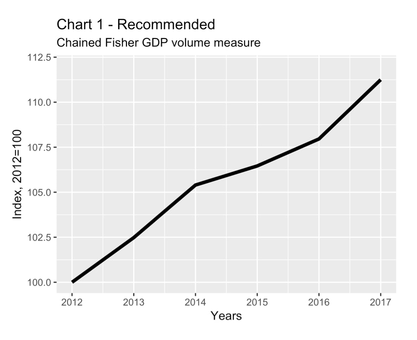
Chart 1 provides an example of a good chart that reflects these principles. It shows the chained Fisher GDP volume measure, otherwise known as “real GDP” or “GDP measured in chained (2007) dollars”, as an index starting at 100 in the first year being examined. The statistics in this chart come from the Statistics Canada table (36-10-0104-01) and they are reported there as being measured in chained (2007) dollars, but to avoid confusion they are shown in the chart after have been rescaled to equal 100 in 2012.
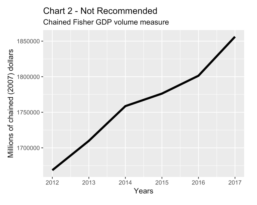
Chart 2 is an example of a type of chart that is not recommended. It shows the same basic information that is in Chart 1, but expressed in chained (2007) dollars instead of in index form. The chart is not wrong - it is simply a plot of the official numbers published by Statistics Canada - but it encourages the viewer to think of the line as representing amounts of a currency called chained (2007) dollars when, in fact, such a currency has no real meaning. It is preferable, and more informative, to show an index number scale on the y-axis with 2012=100, or some other reference year. By scaling to 100 in the initial year, as in Chart 1, the cumulative growth percentage over the period is shown.
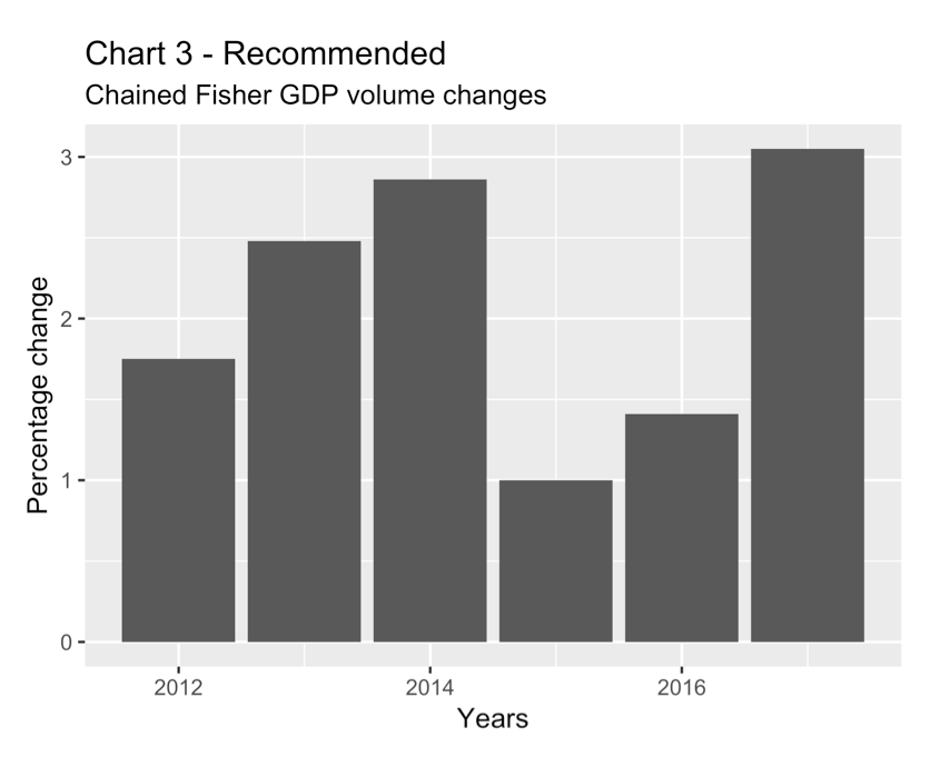
Chart 3 is a simple, recommended chart showing the percentage growth rate of the chained Fisher GDP volume index. The level issues affecting Chart 2 do not apply because the chart shows relative changes rather than levels. This is the type of chart normally used in the Income and Expenditure Accounts Daily releases. By the way, it is important that the changes be relative (percentage) changes. Simple (non-relative) changes are again not recommended because their scale is arbitrary.
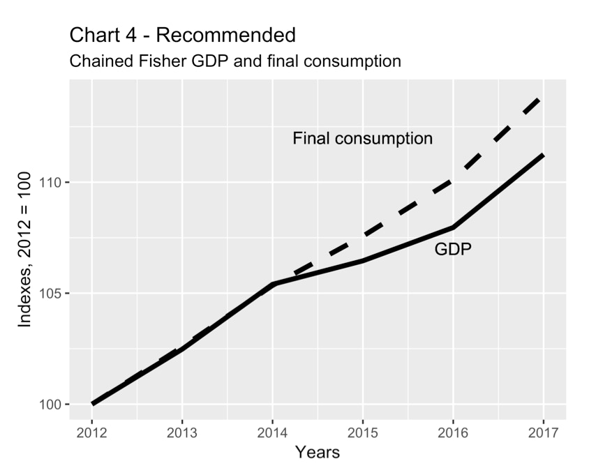
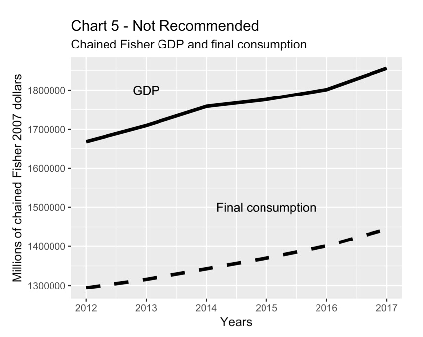
Charts 4 and 5 show two depictions of the volume of final consumption expenditure and GDP. Chart 4 is the recommended version, in which both series have been indexed to equal 100 in 2012. It shows that the two series moved more-or-less in tandem from 2012 to 2014 and then diverged, with final consumption expenditure volume growing more rapidly on a cumulative basis. Chart 5, which is not recommended, depicts the same information but the two series are shown as recorded in Table 36-10-0104-01, measured in chained (2007) dollars. The problem with this chart is that it implies the levels of the two index series are comparable when, in fact, they really are not. Moreover, Chart 4 is more informative because it shows the cumulative percentage change.
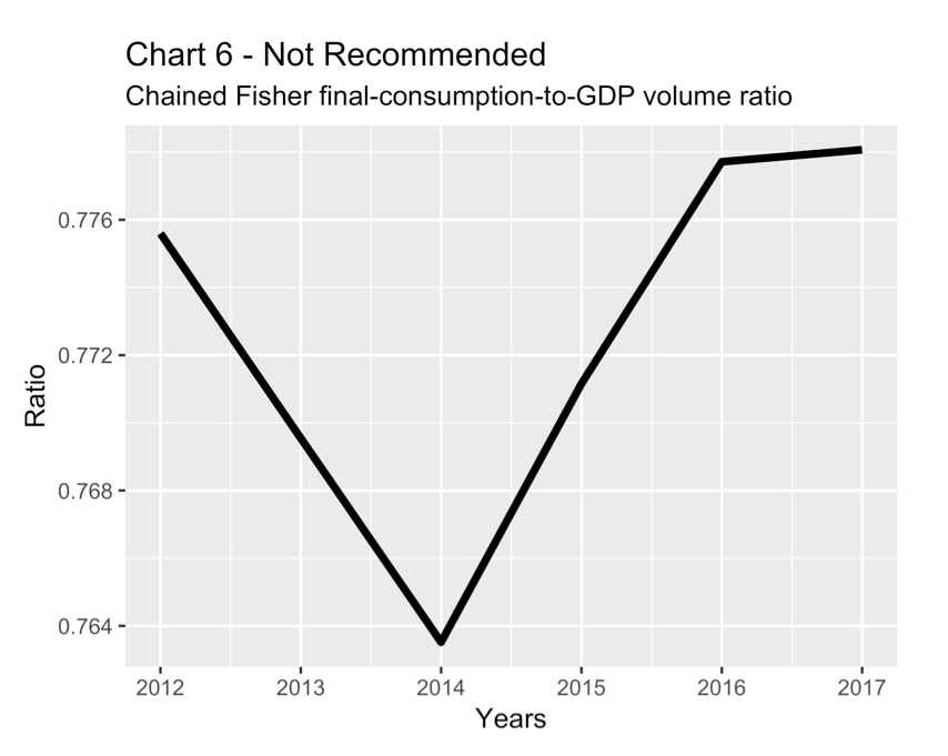
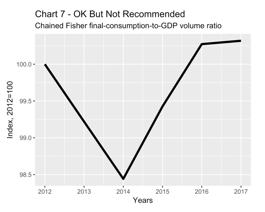
Charts 6 and 7 show two versions of the ratio of the volume of final consumption expenditure to that of GDP. The lines on the two charts have the identical shape but their scales are different. Chart 6 is not recommended because the ratios that are shown on the y-axis are misleading. Chart 7 is better because the axis has been rescaled to highlight its arbitrary nature. But Chart 7 is still not recommended. In this case, it is usually better to show the ratio of the two current dollar series instead of the two volume indexes, as in Chart 8.
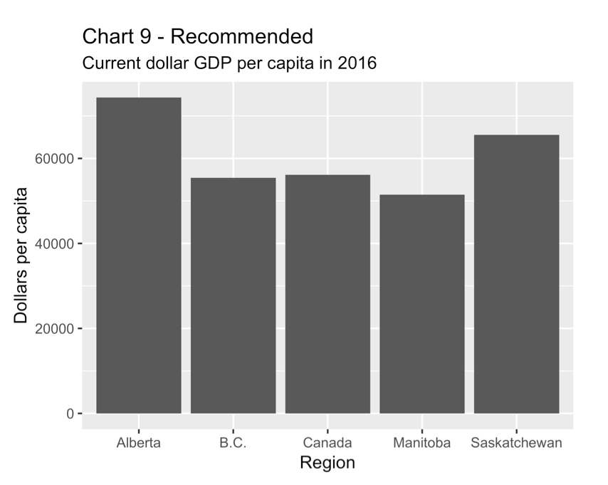
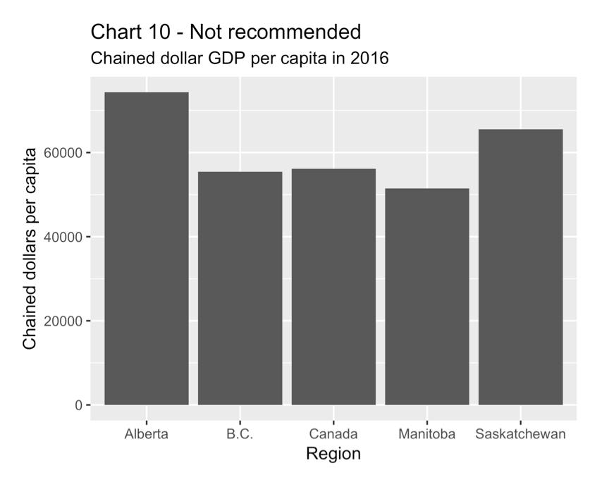
Finally, Charts 9 and 10 show two versions of average GDP per capita, comparing the western provinces to the overall Canada average. The first chart, which is recommended, shows GDP in current dollars divided by population. The second shows GDP in chained dollars divided by population. It is not meaningful to compare chained-dollar GDP per capita, a level, in two regions.
Conclusion
This short note is intended to provide historical context and to clarify what people familiar with index number theory and practice will already know: That the level of a time series in a particular time period, when measured in chained Fisher dollars, is not meaningful. Only the relative changes in a chained-dollar series have a clear interpretation.
References
Chevalier, Michel, [2003] “Chain Fisher Volume Index Methodology,” Statistics Canada, Income and Expenditure Accounts technical series, cat. no. 13-604-MIE, No. 42, Ottawa, November 2003.
Kemp, Katherine and Philip Smith, [1989], “A Technical Note on Laspeyres, Paasche and Chain Price Indexes in the Income and Expenditure Accounts,” National Income and Expenditure Accounts, fourth quarter 1988, Statistics Canada catalogue number 13-001.
Saulnier, Marie, [1990], “Volume indexes in the Income and Expenditure Accounts,” National Income and Expenditure Accounts, first quarter 1990, Statistics Canada catalogue number 13-001.
Wilson, Karen, [1991], “The Introduction of Chain Volume Indexes in the Income and Expenditure Accounts,” National Income and Expenditure Accounts, first quarter 1991, Statistics Canada catalogue number 13-001.
Wilson, Karen, [2001] “Introduction of the Chain Fisher Measure of Real GDP,” Statistics Canada, Latest Developments in the Canadian Economic Accounts, cat. no. 13-605-X, May 2001.